Bring existing wavefunctions and analysis results into Blender. Explore orbitals, density and electrostatic potential, shape the view with native Geometry Nodes, and keep the science with the image.
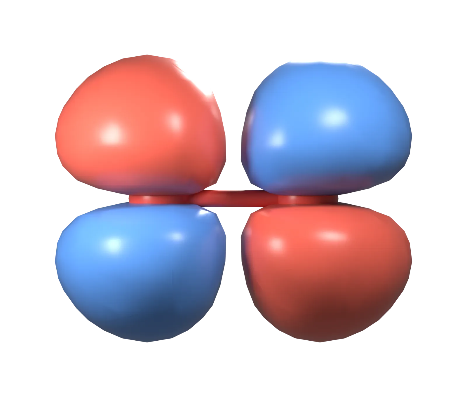
P01 · Molecular orbitalTwo colors represent opposite orbital phases.
In development0.1.0 Alpha
Validated environmentWindows x64 · Blender 5.1.1
Extension availabilityAlpha Preview available
From results to spatial intuition
See the shape. Understand the quantity.
Put molecular structure and spatial fields in one scene. Choose a view around a scientific question, then adjust isovalues, color scales, slices and cameras.
01ORBITALS & DENSITY
Explore orbital shape
and phase in 3D.
Generate molecular orbital and electron density grids from Gaussian FCHK files with a complete basis and MO coefficients, or import existing Cube data. Select an orbital, spin channel and isovalue to compare spatial distributions.
The sign of a real orbital represents phase. Density and orbital amplitude are different physical quantities.
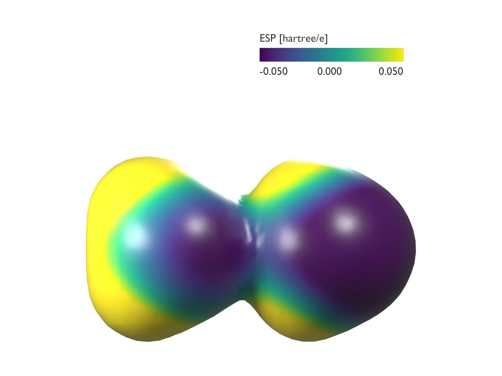
Map ESP onto an electron density surface with a fixed color range and explicit units. Use slices, spatial sampling and line profiles to inspect the numbers behind the colors.
Evaluate supported FCHK data or import existing density and ESP Cube files.
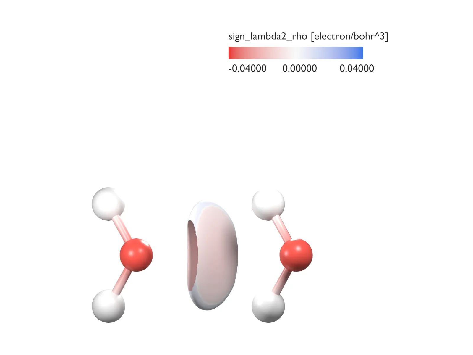
Import paired IGMH / IRI fields computed in external software. Display an isosurface and its coloring field alongside the molecular structure, keeping component, fragment and source declarations with the result.
IGMH / IRI calculations happen in external software. QCBlender reads and displays the results.
Prepare an FCHK, Cube, supported Gaussian/ORCA results or XYZ. Check the physical quantity, units and calculation source.
FCHK / Cube / Gaussian / ORCA OUT・HESS / XYZ
02
Create and adjust a view
Choose an orbital or spatial field. Set isovalues and colors, then add slices, annotations or measurements as needed.
Orbitals · Density · ESP · External analysis
03
Save, render and share
Save a self-contained project, set the camera and lighting, and render with Blender while keeping the relevant parameters.
.blend + .qcdata / Images / Data summaries
Before you begin
Check your environment.
Then open the first example.
QCBlender is in Alpha. The Chinese tutorial starts with installation, a scientific runtime check and the public P01 example, with concrete actions and observable results.
Other platforms and versions have not been validated here. Built-in wavefunction evaluation excludes ECP, complex orbitals and periodic systems. ORCA OUT/HESS supports existing properties and vibrations; GBW, ORCA JSON and .mwfn have no direct importer. See File formats for version and data conditions.
Begin with P01
Make your first
orbital image.
A complete Chinese tutorial takes you from installation to saving a project, with focused topics for the next question.